You may have heard about how array programming languages such as APL, J or K. If you have, you've probably heard that code written in these languages is incredibly dense and unreadable. “Line noise” is a term often used to refer to them.
In this post, I will try to use Kap to give an introduction to the language by using an imperative programming style. Actual Kap code is a mix of terse and verbose styles, but perhaps illustrating the verbose style first provide a different perspective.
If you want to get an introduction to the terse style immediately, you can read the Kap tutorial. Most APL tutorials will also be useful, although there are some differences between Kap and APL (explained here).
This post assumes that the reader has familiarity with various imperative programming languages, such as C, Java or Javascript.
The goal is explain the basic syntax of Kap in a way that is as similar to these programming languages, and then show how adding a little bit of line noise can make expressions much more concise.
Hello world
Let's start with Hello world. It's very simple:
io:println⟦"Hello world"⟧
The double-struck bracket is used when calling a function in an imperative style. This is the same as the parentheses around the arguments to a function in C.
Note: In this particular case, the brackets are optional, but we're getting ahead of ourselves.
While this post is trying to introduce the language in a way so as to make it easier for people without array language familiarity, one still has to accept the use of non-ASCII symbols. If this is something you really cannot get over, then K or Q are probably the languages that would be most suited to your liking.
In any case, I don't think much explanation is needed. Perhaps just worth mentioning that io is the namespace and println is the name of the function.
Assign to a variable
Here's how you assign a value to a variable:
message ← "Hello"
io:println⟦"The message is: ",message⟧
The , is not an argument separator. It's actually a function that concatenates two arrays (strings are just arrays of characters). The resulting string is then printed.
Loop with a counter
Kap features while loops just like most other languages. The syntax is very similar to these languages too:
i ← 0
while (i < 15) {
    io:println⟦"Number: ",⍕i⟧
    i ← i + 1
}
The only unexpected thing here should be the symbol ⍕. This is used to convert number to a string. This conversion isn't strictly necessary here since io:println will automatically convert numbers to strings prior to printing, but I wanted to add it for completeness.
Calling a function with multiple arguments
Just like any other language, Kap allows you to declare functions with multiple arguments. The syntax may be unusual, but it shouldn't be too complicated:
∇ makeCopies (string ; n) {
  result ← ""
  i ← 0
  while ((i←i+1) ≤ n) {
    result ← result,string
  }
  result  ⍝ The return value is the last expression in a function
}
Note how we can modify a variable while using the result. This is exactly the same as in a language like C or Java, except that we have to be explicit since there is no modifying operator. In other words, we have to write i←i+1 rather than ++i (Kap's assignment operator returns the value that was assigned, so the example expression is equivalent to pre-increment).
A ; is used to separate arguments, so we can call the function like so:
makeCopies⟦"zx"; 5⟧
Calling this function will return the string: "zxzxzxzxzx".
Arrays
The primary composite datatype in Kap is the array. An array is just a list of values (exactly like, say, Java) along with a dimensionality (like Common Lisp or Fortan, but unlike Java, Javascript and many other languages). That is to say, while arrays in most languages are indexed using a single integer value, a multidimensional array use multiple integers as an index.
Here's a 1-dimensional array which is assigned to the variable a.
a ← 100 200 300 400
This is an array of 4 elements, and no special syntax is needed to express it. Just listing values separated by whitespace creates a regular array. Compare this to JS, where you would need square brackets and delimiters to do the same thing.
The argument in favour of this syntax is that arrays are such fundamental objects in array languages that they should require an absolute minimum of syntax. (Some other array languages such as BQN disagree here, and require explicit syntax to create arrays)
The above example created a 1-dimensional array. What about higher dimensions? This is easy, but it does force us into the realm of symbols. It's a pretty mild use case though, so it's a good introduction:
b ← 2 2 ⍴ 100 200 300 400
First of all, the symbol ⍴ is the Greek letter “rho”, and it's a function that accepts an argument on either side (just like - accepts an argument to the left, and the value to subtract on the right). In this case, the left argument is the array 2 2, and the right argument is the familiar 4-element list 100 200 300 400 that we saw above.
So what does ⍴ do? Well, it “reshapes” the argument on the right to the dimensionas specified on the left. In this case, it creates new array which is 2 rows by 2 columns, with the values on the right. Typing this into the interpreter will show the following:
┌→──────┐
↓100 200│
│300 400│
└───────┘
Note that this is not a nested array (a 2-element array containing 2 arrays inside it). Instead, it's a single array where each element is indexed using a pair of integers. The pair 0 0 refers to the value 100, the pair 1 0 refers to 300, etc.
The observant reader may have noticed that the ⍴ function specified the total size of the resulting array on the left (in other words, the product of all dimensions) and the array to be reshaped also has a size. What happens if the two don't match?
The reshape operation will take as many elements as it needs, and if there isn't enough, it will start from the beginning. This will become important later when we rewrite the earlier code in a terse way. Here's an example:
    4 2 ⍴ 100 200 300 400
┌→──────┐
↓100 200│
│300 400│
│100 200│
│300 400│
└───────┘
Visualising arrays
2-dimensional arrays are fun and all, but what can you do with them? Let's draw something on the screen. First, we'll create a simple image by generating it as a 1-dimenional array and then we'll reshape it into 2 dimensions so that it can be drawn on the screen.
imgdata ← ⍬  ⍝ This symbol represents the empty list
y ← 0
while (y < 100) {
  x ← 0
  while (x < 100) {
    ⍝ The symbol ⋆ means exponentiation. In other words, the
    ⍝ below expression uses the Pythagorean theorem to compute
    ⍝ the distance of the point from the centre of the screen.
    p ← √((x-50)⋆2)+((y-50)⋆2)
    imgdata ← imgdata,(p÷50)
    x ← x + 1
  }
  y ← y + 1
}
⍝ The resulting array is 1-dimensional, so we reshape
⍝ it into a 100-by-100 array before it can be displayed.
resized ← 100 100 ⍴ imgdata
gui:draw resized
Time for terseness
The above program works, and it's a perfectly acceptable way to write Kap code. However, it doesn't really take advantage of the power of the language. The idea of Kap is that you use it as a very powerful calculator, and in situations like that you don't want to write a 12 line program just to generate that array of numbers.
Let's imagine we're working in the REPL, and we have no intention of saving this program to a file or share it with others. I'm making this initial assumption in order to avoid having a discussion around how to document terse Kap code. That needs to be the topic of a separate post.
Index generator and scalar functions
The power of array programming come from the idea that instead of looping over some set of values, you perform operations that are defined on the entire array at a time. This includes things like mathematical operations (addition, subtraction, etc) and functional operations like mapping and reduction. Most of these core functions are a single character, which makes for a very powerful language, but is also why people tend to think it's “unreadable”.
Note: there are a lot of different ways to approach this problem, and when I was discussing this in the Array Programming Matrix Room, several different approaches were suggested. I've picked the one I will be presenting because I believe it does the best job at highlighting the topics that I'd like to discuss, not necessarily because it's the best solution.
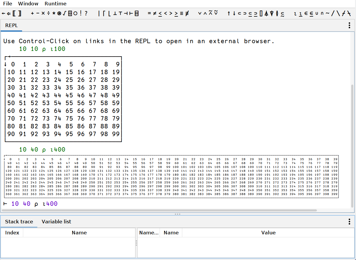
We're going to need the index generator function, so let's start by introducing it. The name is ⍳ (the Greek letter iota), and can be called with one argument, returning an array of indexes into an array of the given dimensions. For example: ⍳10 returns a 1-dimensional array containing the numbers 0 to 9:
    ⍳10
┌→──────────────────┐
│0 1 2 3 4 5 6 7 8 9│
└───────────────────┘
Note: we don't have to use the double-struck brackets to enclose the argument. When an argument is passed without these brackets, everything to the right of the function name constitute the arguments, unless override by parentheses. This means that the above could also have been written as ⍳5+5. I.e. functions are called with right precedence when called without brackets.
Next, we need to discuss scalar functions. These are functions that act on all elements in an array. For example, if we add a number to an array, this is the same as adding that number to every cell in the array. Since we're going to work ourselves up to a terse version of the previous program, let's subtract 5 from ⍳10 (we'll later use 100 and 50):
    (⍳10)-5
┌→───────────────────────┐
│-5 -4 -3 -2 -1 0 1 2 3 4│
└────────────────────────┘
Note: we use parens around ⍳10 because of the aforementioned right precedence. If we skip the parens we end up with the equivalent of ⍳(10-5).
Now, if we reshape this thing to a 10-by-10 array, we end up with an array that contains the x-coordinates of the pixels. Let's assign it to a variable because we'll need it later:
    xcoords ← 10 10 ⍴ (⍳10)-5
┌→───────────────────────┐
↓-5 -4 -3 -2 -1 0 1 2 3 4│
│-5 -4 -3 -2 -1 0 1 2 3 4│
│-5 -4 -3 -2 -1 0 1 2 3 4│
│-5 -4 -3 -2 -1 0 1 2 3 4│
│-5 -4 -3 -2 -1 0 1 2 3 4│
│-5 -4 -3 -2 -1 0 1 2 3 4│
│-5 -4 -3 -2 -1 0 1 2 3 4│
│-5 -4 -3 -2 -1 0 1 2 3 4│
│-5 -4 -3 -2 -1 0 1 2 3 4│
│-5 -4 -3 -2 -1 0 1 2 3 4│
└────────────────────────┘
Now, if we transpose this array using the function ⍉, we get the y-coordinates, which we then assign to another variable:
    ycoords ← ⍉xcoords
┌→────────────────────────────┐
↓-5 -5 -5 -5 -5 -5 -5 -5 -5 -5│
│-4 -4 -4 -4 -4 -4 -4 -4 -4 -4│
│-3 -3 -3 -3 -3 -3 -3 -3 -3 -3│
│-2 -2 -2 -2 -2 -2 -2 -2 -2 -2│
│-1 -1 -1 -1 -1 -1 -1 -1 -1 -1│
│ 0  0  0  0  0  0  0  0  0  0│
│ 1  1  1  1  1  1  1  1  1  1│
│ 2  2  2  2  2  2  2  2  2  2│
│ 3  3  3  3  3  3  3  3  3  3│
│ 4  4  4  4  4  4  4  4  4  4│
└─────────────────────────────┘
We can square the entire array simply by using ⋆ since it's a scalar function:
    ycoords⋆2
┌→────────────────────────────┐
↓25 25 25 25 25 25 25 25 25 25│
│16 16 16 16 16 16 16 16 16 16│
│ 9  9  9  9  9  9  9  9  9  9│
│ 4  4  4  4  4  4  4  4  4  4│
│ 1  1  1  1  1  1  1  1  1  1│
│ 0  0  0  0  0  0  0  0  0  0│
│ 1  1  1  1  1  1  1  1  1  1│
│ 4  4  4  4  4  4  4  4  4  4│
│ 9  9  9  9  9  9  9  9  9  9│
│16 16 16 16 16 16 16 16 16 16│
└─────────────────────────────┘
We can now put the entire thing together:
(√ (ycoords⋆2) + (xcoords⋆2)) ÷ 5
(I'm not including the output of this operation, since the array is pretty big. Suffice it to say that it does contain the numbers we're looking for)
We're not done making the program terse yet, but below is the entire program as it stands right now:
xcoords ← 100 100 ⍴ (⍳100)-50
ycoords ← ⍉xcoords
gui:draw (√(ycoords⋆2) + (xcoords⋆2)) ÷ 50
Let's compress this thing further
The program above is much closer to what you'd end up writing on the REPL, especially if it's the result of some experimentation so that you'd have these arrays in variables already. When writing it from scratch, however, you probably want to type even less, so let's use some powerful features of Kap that allows you to be even more terse.
Kap allows you to write inline functions using { and }. The code between the braces is a function in itself, with the left and right arguments being assigned to the variables ⍺ and ⍵. While there are many ways in which inline functions (or dfns, as they are usually called) can be used, one use case is to provide an efficient way to evaluate some code with an expression assigned to a variable, without having to assign and name said variable separately. This is very useful in the example below, since the 100-by-100 array we created first is needed twice inside the dfn. We then inline the call to ⍉ since there is no need to store that in a separate variable:
gui:draw { (√(⍵⋆2) + ((⍉⍵)⋆2)) ÷ 50 } 100 100 ⍴ (⍳100)-50
You can of course go even further. There are several repetitions in the code above, but unless we're doing code golf, there really isn't much reason to go that far. I've also intentionally avoided using a lot of features that would be quite useful here, mainly because the post is already pretty long, and such descriptions are more useful if it's part of a separate post.
It may also be of interest that the above version does not actually create several arrays of pixel data. These arrays are represented internally as abstract objects and they are not actually realised into data until the final pixmap is generated in the gui:draw function.
Terse version of the string duplication function
For completeness sake, here's one way you could write the makeCopies function above. It only uses one new function that hasn't been talked about yet: ≢, which returns the size of its argument.
Actually, you'd probably not even put it in a function, but rather just inline it:
5 { (⍺×≢⍵) ⍴ ⍵ } "xz"
Further reading
The main Kap website is perhaps not the most beautiful website, but might contain some interesting information for people who got all the way to the end of this post.
More code examples can be found on the Kap examples page.